As we consider the wide set of things in the world that we would like to represent in our programs, we find that most of them have compound structure. For example, a geographic position has latitude and longitude coordinates. A date has a year, month, and day. Introducing dedicated types to represent concepts in the world, such as positions and dates, has proven to be an excellent way to organize complex programs.
The Object Metaphor
An object combines values and behavior. The central characteristic of objects is that they represent information but also behave like the information that they represent. When an object is printed, it provides text to describe itself. If an object is a combination of parts, it provides access to those parts. Objects are both information and functionality, bundled together to provide abstract representations.
In Python, all values are objects. Rather than data consisting of only numbers manipulated by functions, data are objects that have types which endow those objects with behavior. Python’s date type provides an excellent illustration. While a program could use a list of integers (a year, month, and day) to represent a date, a date object bundles in a great deal of date-related functionality.
>>> from datetime import date
>>> date
<class 'datetime.date'>
>>> final = date(2026, 12, 18)
>>> final
datetime.date(2026, 12, 18)
The name date is bound to a class, which represents a kind of value. Individual dates are called instances or objects of that class. Instances are constructed by calling the class on arguments that describe the instance.
While final was constructed from primitive numbers, it behaves like a date. For instance, subtracting it from another date will give a time difference, which we can print.
>>> print(date(2026, 12, 21) - final)
3 days, 0:00:00
Objects have attributes, which are named values that are part of the object. In Python, like many other programming languages, we use dot notation to designate an attribute of an object.
<expression> . <name>
Above, the <expression> evaluates to an object, and <name> is the name of an attribute for that object.
Attribute names are not available in the global environment. Instead, they are particular to the object instance preceding the dot.
>>> final.year
2026
>>> final.day
18
Objects also have methods, which are function-valued attributes. Metaphorically, we say that the object “knows” how to carry out those methods. By implementation, methods are functions that compute their results from both their arguments and their object. For example, the strftime method (an abbreviation for “string format of time”) of final takes a single argument that specifies how to display a date (e.g., %A means that the day of the week should be spelled out in full).
>>> final.strftime('%A, %B %d')
'Friday, December 18'
Computing the return value of strftime requires two inputs: the string that describes the format of the output and the date information bundled into final. Date-specific logic is applied within this method to yield this result. We never stated that the 18th of December, 2026, was a Friday, but knowing the corresponding weekday is part of what it means to be a date. By bundling behavior and information together, this Python object offers us a convincing, self-contained abstraction of a date.
Dates are objects, but numbers, strings, lists, and ranges are all objects as well. They represent values, but also behave in a manner that befits the values they represent. They also have attributes and methods. For instance, strings have several methods that facilitate text processing.
>>> '1234'.isnumeric()
True
>>> 'rOBERT dE nIRO'.swapcase()
'Robert De Niro'
>>> 'eyes'.upper().endswith('YES')
True
Data Classes
To represent positions as objects, we would like our programming language to have the capacity to introduce a new class, the Position, which couples together a latitude and longitude into a compound object that our programs can manipulate as a single conceptual unit, but which also has two coordinates that can be accessed using dot expressions.
We could use a two-element list to represent a position, but then we would have to remember whether the latitude or longitude came first everywhere that we want to access its coordinates.
We can instead create a Position type that has attributes called lat and lon using a class statement with a dataclass decorator. The class statement is used to create new user-defined types. Many more details of class statements will be described in Section 2.5 on object-oriented programming. The dataclass decorator simplifies the creation of classes for compound data. The lines indented below the class header declare that every Position object has two attributes lat and lon that are intended to be numbers.
>>> from dataclasses import dataclass

>>> @dataclass
    class Position:
        "A geographic position."
        lat: float
        lon: float
Once this class statement is executed, new Position objects can be created by calling Position on a pair of numbers. The coordinates of a position are accessed using dot expressions.
>>> sydney = Position(-33.87, 151.21)
>>> sydney.lat
-33.87
>>> sydney.lon
151.21
>>> sydney
Position(lat=-33.87, lon=151.21)
>>> type(sydney) == Position
True
>>> isinstance(sydney, Position)
True
A Position can be formatted to include cardinal directions (N, S, E, W) by defining a function that takes a Position and returns a str. [1]
>>> def format_pos(p: Position) -> str:
        "Format the position as a string with directional suffixes."
        assert abs(p.lat) <= 90 and abs(p.lon) <= 180, f'{p!r} is not on Earth!'
        if p.lat >= 0:
            lat_dir = "N"
        else:
            lat_dir = "S"

        if p.lon >= 0:
            lon_dir = "E"
        else:
            lon_dir = "W"

        return f"{abs(p.lat)}° {lat_dir}, {abs(p.lon)}° {lon_dir}"

>>> format_pos(sydney)
'33.87° S, 151.21° E'
We can redefine the Position class to include a __str__ method, which is a function defined within a class. This special name __str__ directs Python to call format_pos each time any Position is printed or passed to str. A full description of how to add behavior to classes appears in Section 2.5 on object-oriented programming. For now, we will focus on ensuring that our user-defined data types provide useful information when printed.
>>> @dataclass
    class Position:
        "A geographic position."
        lat: float
        lon: float

        def __str__(self):
            return format_pos(self)
>>> sydney = Position(-33.87, 151.21)
>>> str(sydney)
'33.87° S, 151.21° E'
>>> print('The position of Sydney is', sydney)
The position of Sydney is 33.87° S, 151.21° E
Data Abstraction
Before continuing with further examples of user-defined types, it is worth observing the role of abstraction in the position example. By defining a class, we can use a Position---accessing its named attributes (lat and lon) or printing it---without needing to specify or decide how its primitive components are stored and combined. Without using a class statement, we would need to decide whether a position is represented as a list, a dictionary, or some other way, and each time we wanted to print a position we would need to call format_pos.
In fact, all the native classes we have used are also abstractions. A Python list has some way in which its items are stored and combined, but we can use a list---accessing its length and items---without reasoning about its representation in the computer’s memory. We can print a list without thinking about the process that constructs its printed representation. Likewise, dictionaries and strings are abstractions that allow us to interact with compound data while abstracting away the details of exactly how a dictionary looks up a value by its key or how a string can represent letters in many different alphabets. Even int and float types are abstractions that allow us to work with numbers without always reasoning about the details of how numbers are stored by the transistors of a computer.
Data abstraction involves giving a name to a type of data and interacting with compound data values according to a fixed set of operations that are specific to that type of data, without making assumptions or reasoning about how those operations are implemented. It is analogous to functional abstraction, which involves giving a name to a computational process and using it (by calling a function) without making assumptions or reasoning about how the process is implemented.
Eventually learning about the implementation of data abstractions is both interesting and important for building useful software. But it is also helpful to learn to work with data abstractly. Expert programmers not only understand how numbers, lists, dictionaries, and classes are implemented, but also learn to use these types of objects without always thinking about their implementation. The concept of an object, which is shared by many programming languages, is designed to help separate the use and implementation of compound data.
Linked Lists
So far, we have used only native types to represent sequences. However, we can also develop sequence representations that are not built into Python. For example, a common and useful representation of a sequence is the linked list.
A linked list combines a first item of a sequence and the rest of the sequence. Linked lists have a recursive structure: the rest of a linked list is another linked list. It is possible to represent a linked list just with two-element tuples, using the empty tuple to represent an empty linked list. In this way, we see that any method of combining two values can be used to represent a sequence of any length.
Linked lists differ from two-item tuples because of their regular structure: each first item has the same type and each second item is another linked list. We can express this structure using a data class for linked lists.
>>> type LinkedList[T] = Link[T] | tuple[()]

>>> @dataclass
    class Link[T]:
        "A Link has a first value of type T and the rest of the linked list."
        first: T
        rest: LinkedList[T] = ()  # rest defaults to an empty linked list
The type tuple[()] has only one compatible value: the empty tuple.
The examples below demonstrate how to construct a linked list containing the numbers 3, 4, and 5 and how to access its items using first and rest attributes.
>>> s = Link(3, Link(4, Link(5)))
>>> s.first
3
>>> s.rest.first
4
>>> s.rest.rest.first
5
>>> s.rest.rest.rest == ()
True
>>> s
Link(first=3, rest=Link(first=4, rest=Link(first=5, rest=())))
>>> s.rest.rest
Link(first=5, rest=())
There is no one standardized way to display a linked list, but a common one is to show the items it contains within parentheses and without commas. This notation was introduced by the Lisp programming language, one of the oldest languages still widely used today.
Adding a __str__ method to the Link class generates this string representation each time a Link object is printed or passed to str.
>>> def format_link(s: Link):
        """Return a Link s formatted as items within parentheses."""
        string = '(' + str(s.first)
        remaining = s.rest
        while isinstance(remaining, Link):
            string += ' ' + str(remaining.first)
            remaining = remaining.rest
        assert remaining == (), f'{s!r} is not a LinkedList'
        return string + ')'
>>> @dataclass
    class Link[T]:
        "A Link has a first value of type T and the rest of the linked list."
        first: T
        rest: LinkedList[T] = ()  # rest defaults to an empty linked list

        def __str__(self):
            return format_link(self)
>>> s = Link(3, Link(4, Link(5)))
>>> print(s)
(3 4 5)
The complete Link class appears in the examples appendix.
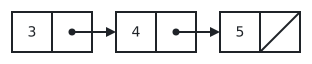
The most common way to visualize any linked list, whether created from tuples or a data class, is to use a box-and-pointer diagram in which each Link is a pair of boxes holding its first and rest and the empty list is denoted by a slash through the rest of the final Link in a linked list. Here is the diagram for Link(3, Link(4, Link(5))), which would be printed as (3 4 5).
Here are two example functions that take linked lists: len_link returns the number of items contained in a linked list and getitem_link returns an item by its position.
>>> def len_link(s: LinkedList):
        """Return the length of a linked list."""
        length = 0
        while isinstance(s, Link):
            length += 1
            s = s.rest
        return length
>>> len_link(s)
3

>>> def getitem_link(s: LinkedList, i: int):
        """Return the item at index i of a non-empty linked list."""
        while i > 0:
            assert isinstance(s, Link), 'Index out of range'
            s = s.rest
            i -= 1
        assert isinstance(s, Link), 'Index out of range'
        return s.first
>>> getitem_link(s, 1)
4
Type variables. Like a list, a LinkedList typically holds items that all share a type. The LinkedList[T] and Link[T] types have a type variable T, which represents a shared type for all of the items they contain. It can be replaced by any type. For example, a LinkedList[int] describes a LinkedList that contains int values as all of its items. Functions that take or return linked lists can optionally specify the type of items contained within those lists.
>>> def sum_link(s: LinkedList[float]) -> float:
        """Return the sum of the items in a linked list of numbers."""
        total = 0
        while isinstance(s, Link):
            total += s.first
            s = s.rest
        return total
>>> sum_link(s)
12
These examples demonstrate a common pattern of computation with linked lists, where each step in an iteration operates on an increasingly shorter suffix of the original list.
Recursive manipulation. len_link, getitem_link, and sum_link are iterative. They peel away each Link until the end of the list (in len_link and sum_link) or the desired item (in getitem_link) is reached. We can also implement all three using recursion.
>>> four = Link(1, Link(2, Link(3, Link(4))))
>>> print(four)
(1 2 3 4)
>>> def len_link_recursive(s: LinkedList) -> int:
        """Return the length of a linked list s."""
        if not isinstance(s, Link):
            return 0
        return 1 + len_link_recursive(s.rest)
>>> len_link_recursive(four)
4

>>> def getitem_link_recursive(s: LinkedList, i: int):
        """Return the item at index i of linked list s."""
        assert isinstance(s, Link), 'Index out of range'
        if i == 0:
            return s.first
        return getitem_link_recursive(s.rest, i - 1)
>>> getitem_link_recursive(four, 1)
2

>>> def sum_link_recursive(s: LinkedList[float]) -> float:
        """Return the sum of the items in a linked list of numbers."""
        if not isinstance(s, Link):
            return 0
        return s.first + sum_link_recursive(s.rest)
>>> sum_link_recursive(s)
12
Recursion is also useful for transforming and combining linked lists.
>>> def extend_link(s: LinkedList, t: LinkedList) -> LinkedList:
        """Return a linked list with the items of s followed by those of t."""
        if not isinstance(s, Link):
            return t
        else:
            return Link(s.first, extend_link(s.rest, t))

>>> print(extend_link(four, four))
(1 2 3 4 1 2 3 4)

>>> def apply_to_all_link(f, s: LinkedList) -> LinkedList:
        """Return a linked list of f applied to each item of s."""
        if not isinstance(s, Link):
            return s
        else:
            return Link(f(s.first), apply_to_all_link(f, s.rest))

>>> print(apply_to_all_link(lambda x: x*x, four))
(1 4 9 16)

>>> def keep_if_link(f, s: LinkedList) -> LinkedList:
        """Return a linked list with the items of s for which f returns a true value."""
        if not isinstance(s, Link):
            return s
        else:
            kept = keep_if_link(f, s.rest)
            if f(s.first):
                return Link(s.first, kept)
            else:
                return kept

>>> print(keep_if_link(lambda x: x%2 == 0, four))
(2 4)

>>> def join_link(s: LinkedList, separator: str) -> str:
        """Return a string of all items in s separated by separator."""
        if not isinstance(s, Link):
            return ""
        elif not isinstance(s.rest, Link):
            return str(s.first)
        else:
            return str(s.first) + separator + join_link(s.rest, separator)

>>> print(join_link(four, ", "))
1, 2, 3, 4
Recursive construction. Linked lists are particularly useful when constructing sequences incrementally, a situation that arises often in recursive computations.
The count_partitions function from Chapter 1 counted the number of ways to partition an integer n using parts up to size m via a tree-recursive process. With sequences, we can also enumerate these partitions explicitly using a similar process.
We follow the same recursive analysis of the problem as we did while counting: partitioning n using integers up to m involves either
partitioning
n-musing integers up tom, orpartitioning
nusing integers up tom-1.
For base cases, we find that 0 has one partition that is empty, while partitioning a negative integer or using parts smaller than 1 is impossible.
>>> def partitions(n: int, m: int) -> list[LinkedList[int]]:
        """Return a list of partitions of n using parts of up to m.
        Each partition is represented as a linked list.
        """
        if n == 0:
            return [()] # A list containing the empty partition
        elif n < 0 or m == 0:
            return []
        else:
            with_m = [Link(m, s) for s in partitions(n-m, m)]
            without_m = partitions(n, m-1)
            return with_m + without_m
In the recursive case, we construct two sublists of partitions. The first uses m, and so we prepend m to each item returned by the recursive call partitions(n-m, m) to form with_m. This use of linked lists is more efficient than using native Python lists because prepending can be achieved just by constructing one new Link.
The result of partitions is a (regular Python) list of linked lists. Using join_link, we can display each partition in a human-readable manner.
>>> def print_partitions(n: int, m: int) -> None:
        "Print the partitions of n using parts up to size m."
        for p in partitions(n, m):
            print(join_link(p, " + "))
>>> print_partitions(6, 4)
4 + 2
4 + 1 + 1
3 + 3
3 + 2 + 1
3 + 1 + 1 + 1
2 + 2 + 2
2 + 2 + 1 + 1
2 + 1 + 1 + 1 + 1
1 + 1 + 1 + 1 + 1 + 1
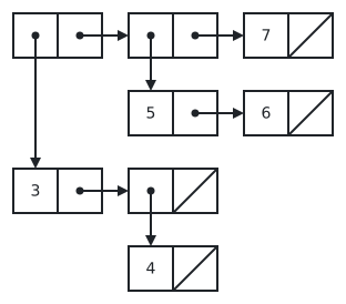
Nested linked lists. The first item in a linked list can be any object, including another linked list. Nested structures can be created by placing linked lists within linked lists, and box-and-pointer diagrams are useful for visualizing these structures. Here is the diagram for Link(Link(3, Link(Link(4))), Link(Link(5, Link(6)), Link(7))), which would be printed as ((3 (4)) (5 6) 7).
Trees
Nesting lists within lists is a way to create hierarchical structures, but the tree is a fundamental data abstraction that imposes regularity on how hierarchical values are structured and manipulated.
A tree has a root label (which can be any value) and a sequence of branches. Each branch of a tree is a tree. A tree with no branches is called a leaf. Any tree contained within a tree is called a sub-tree of that tree (such as a branch of a branch). The root of each sub-tree of a tree is called a node in that tree.
Here is a simple data class for a Tree.
>>> from __future__ import annotations  # for Python 3.12 and 3.13
>>> from dataclasses import field
>>> @dataclass
    class Tree[T]:
        "A Tree has a label (of type T) and a list of branches, which are trees."
        label: T
        branches: list[Tree[T]] = field(default_factory=list)  # branches defaults to []
For Python versions 3.12 and 3.13, executing from __future__ import annotations before this definition is necessary to allow a Tree to contain a list[Tree[T]] attribute using this type hint syntax. For Python 3.14 and later, this import is unnecessary.
The complicated expression field(default_factory=list) is required to provide a default empty list value for the branches attribute, rather than just [], due to the concept of mutation that will be discussed in Section 2.4. This expression ensures that each leaf gets its own empty list of branches rather than sharing the same list with other Tree objects.
Trees can be constructed by nested expressions. The following Tree object t has root label 3 and two branches.
>>> t = Tree(3, [Tree(1), Tree(2, [Tree(1), Tree(1)])])
>>> t.branches[0]
Tree(label=1, branches=[])
>>> len(t.branches)
2
>>> t.branches[1].label
2
>>> len(t.branches[1].branches)
2
Here we introduce a string representation that shows all of the labels within the tree indented to show how deep within the tree’s branches they appear. The newly added __str__ method of the Tree class ensures that format_tree will be called whenever a Tree object is printed or passed to str.
>>> def format_tree(t: Tree, indent='') -> str:
        "Format a tree with each branch indented below its label."
        assert isinstance(t, Tree), f'{t!r} is not a Tree'
        assert isinstance(t.branches, list), f'branches of {t!r} is not a list'
        string = indent + str(t.label)
        for b in t.branches:
            string += '\n' + format_tree(b, indent + '  ')
        return string
>>> @dataclass
    class Tree[T]:
        "A Tree has a label (of type T) and a list of branches, which are trees."
        label: T
        branches: list[Tree[T]] = field(default_factory=list)  # branches defaults to []

        def __str__(self):
            return format_tree(self)
The is_leaf function takes a Tree and returns whether it is a leaf. It makes programs that use trees easier to follow.
def is_leaf(t: Tree) -> bool:
    "Return whether a Tree t is a leaf with no branches."
    return not t.branches
The complete Tree class appears in the examples appendix.
The example below constructs a tree representing the evaluation of the expression ((2 * 3) + 4).
>>> expr = Tree(10, [Tree(6, [Tree(2), Tree('*'), Tree(3)]), Tree('+'), Tree(4)])
>>> print(expr)
10
  6
    2
    *
    3
  +
  4
The Tree Abstraction
Trees are used to represent a variety of hierarchical structures, such as the organizational charts of institutions, the structure of web pages, and even Python code. There are two complementary and compatible ways to view a tree. The recursive description matches our Tree class and uses arboreal terminology: trees have branches and leaves.
A tree can also be described as a collection of nodes, which are the Tree objects. Each node has a label and relations to other nodes. Genealogical terminology applies to this description: the parent of a node is the Tree that contains it as a branch, and the children of a node are the Tree objects in its list of branches. The ancestors of a node include its parent and the parent of any ancestor. The descendants of a node include its children and any children of its descendants.
Both ways of describing a tree use the term root to describe the Tree object that contains the entire tree, and the root label is the label of that object.
A tree is typically visualized by placing each label in a node and drawing an arrow to each child node. The root node is at the top.
![Diagram of the tree Tree(label=10, branches=[Tree(label=6, branches=[Tree(label=2, branches=[]), Tree(label='*', branches=[]), Tree(label=3, branches=[])]), Tree(label='+', branches=[]), Tree(label=4, branches=[])])](/3ed/build/bb0b6c19cad459b01dd2e422f29ec3b5.svg)
Tree-Recursive Functions
Tree-recursive functions can be used to construct trees. For example, the nth Fibonacci tree has a root label of the nth Fibonacci number and, for n > 1, two branches that are also Fibonacci trees. A Fibonacci tree illustrates the tree-recursive computation of a Fibonacci number.
>>> def fib_tree(n: int) -> Tree[int]:
        if n == 0 or n == 1:
            return Tree(n)
        else:
            left, right = fib_tree(n-2), fib_tree(n-1)
            fib_n = left.label + right.label
            return Tree(fib_n, [left, right])
>>> print(fib_tree(5))
5
  2
    1
    1
      0
      1
  3
    1
      0
      1
    2
      1
      1
        0
        1
This fib_tree(5) object can be described recursively: a Fibonacci tree has a Fibonacci number as its label and two Fibonacci trees as its branches. Its contents can also be described in terms of its node relations: the label of each node in a Fibonacci tree is the sum of the labels of its children.
Tree-recursive functions are also used to process trees. For example, the sum_leaves function sums the labels of the leaves of a tree.
>>> def sum_leaves(t: Tree) -> int:
        if is_leaf(t):
            return t.label
        else:
            branch_sums = [sum_leaves(b) for b in t.branches]
            return sum(branch_sums)
>>> sum_leaves(Tree(5, [Tree(100), Tree(1000, [Tree(3), Tree(20)])]))
123
>>> sum_leaves(fib_tree(5))
5
>>> sum_leaves(fib_tree(6))
8The
f'{p!r} ...'syntax directs the f-string to use the built-in representation for aPositionrather than the one defined byformat_pos. This directive ensures that generating the error message withinformat_poswon’t trigger another call toformat_posonce we installformat_posas the function that generates the output of callingstrorprinton aPosition.