2.9 Efficiency

from pytutor import env_diagram

Decisions of how to represent and process data are often influenced by the efficiency of alternatives. Efficiency refers to the computational resources used by a representation or process, such as how much time and memory are required to compute the result of a function or represent an object. These amounts can vary widely depending on the details of an implementation.

Measuring Efficiency¶

Measuring exactly how long a program requires to run or how much memory it consumes is challenging, because the results depend upon many details of how a computer is configured. A more reliable way to characterize the efficiency of a program is to measure how many times some event occurs, such as a function call.

Let’s return to our first tree-recursive function, the fib function for computing numbers in the Fibonacci sequence.

>>> def fib(n):
        if n == 0:
            return 0
        if n == 1:
            return 1
        return fib(n-2) + fib(n-1)

>>> fib(5)
5

Consider the pattern of computation that results from evaluating fib(5), depicted below. To compute fib(5), we compute fib(3) and fib(4). To compute fib(3), we compute fib(1) and fib(2). In general, the evolved process looks like a tree. Each blue dot indicates a completed computation of a Fibonacci number in the traversal of this tree.

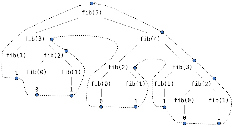
This function is instructive as a prototypical tree recursion, but it is a terribly inefficient way to compute Fibonacci numbers because it does so much redundant computation. The entire computation of fib(3) is duplicated, and fib(2) is computed three separate times.

We can measure this inefficiency. The higher-order count function returns an equivalent function to its argument that also maintains a call_count attribute. In this way, we can inspect just how many times fib is called.

>>> def count(f):
        def counted(*args):
            counted.call_count += 1
            return f(*args)
        counted.call_count = 0
        return counted

By counting the number of calls to fib, we see that the number of calls required grows faster than the Fibonacci numbers themselves. This rapid expansion of calls is characteristic of tree-recursive functions.

>>> fib = count(fib)
>>> fib(19)
4181
>>> fib.call_count
13529

Space. To understand the space requirements of a function, we must specify generally how memory is used, preserved, and reclaimed in our environment model of computation. In evaluating an expression, the interpreter preserves all active environments and all values and frames referenced by those environments. An environment is active if it provides the evaluation context for some expression being evaluated. An environment becomes inactive whenever the function call for which its first frame was created finally returns.

For example, when evaluating fib, the interpreter proceeds to compute each value in the order shown previously, traversing the structure of the tree. To do so, it only needs to keep track of those nodes that are above the current node in the tree at any point in the computation. The memory used to evaluate the rest of the branches can be reclaimed because it cannot affect future computation. In general, the space required for tree-recursive functions will be proportional to the maximum depth of the tree.

The diagram below depicts the environment created by evaluating fib(2). In the process of evaluating the return expression for the initial application of fib, the expression fib(n-2) is evaluated, yielding a value of 0. Once this value is computed, the corresponding environment frame (grayed out) is no longer needed: it is not part of an active environment. Thus, a well-designed interpreter can reclaim the memory that was used to store this frame. On the other hand, if the interpreter is currently evaluating fib(n-1), then the environment created by this application of fib (in which n is 1) is active. In turn, the environment originally created to apply fib to 2 is active because its return value has not yet been computed.

env_diagram(r'''
def fib(n):
    if n == 0:
        return 0
    if n == 1:
        return 1
    return fib(n-2) + fib(n-1)

result = fib(2)
''', step=8, cumulative=True)

The higher-order count_frames function tracks open_count, the number of calls to the function f that have not yet returned. The max_count attribute is the maximum value ever attained by open_count, and it corresponds to the maximum number of frames that are ever simultaneously active during the course of computation.

>>> def count_frames(f):
        def counted(*args):
            counted.open_count += 1
            counted.max_count = max(counted.max_count, counted.open_count)
            result = f(*args)
            counted.open_count -= 1
            return result
        counted.open_count = 0
        counted.max_count = 0
        return counted

>>> fib = count_frames(fib)
>>> fib(19)
4181
>>> fib.open_count
0
>>> fib.max_count
19
>>> fib(24)
46368
>>> fib.max_count
24

To summarize, the space requirement of the fib function, measured in active frames, is equal to the input, which tends to be small. The time requirement measured in total recursive calls is larger than the output, which is huge even for small inputs.

Memoization¶

Tree-recursive computational processes can often be made more efficient through memoization, a powerful technique for increasing the efficiency of recursive functions that repeat computation. A memoized function will store the return value for any arguments it has previously received. A second call to fib(25) would not re-compute the return value recursively, but instead return the existing one that has already been constructed.

Memoization can be expressed naturally as a higher-order function, which can also be used as a decorator. The definition below creates a cache of previously computed results, indexed by the arguments from which they were computed. The use of a dictionary requires that the argument to the memoized function be immutable.

>>> def memo(f):
        cache = {}
        def memoized(n):
            if n not in cache:
                cache[n] = f(n)
            return cache[n]
        return memoized

If we apply memo to the recursive computation of Fibonacci numbers, a new pattern of computation evolves, depicted below.

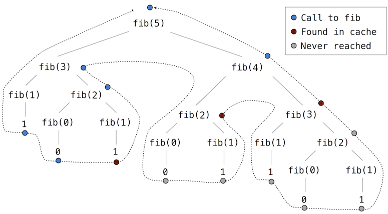
In this computation of fib(5), the results for fib(2) and fib(3) are reused when computing fib(4) on the right branch of the tree. As a result, much of the tree-recursive computation is not required at all.

Using count, we can see that the fib function is actually only called once for each unique input to fib.

>>> counted_fib = count(fib)
>>> fib = memo(counted_fib)
>>> fib(19)
4181
>>> counted_fib.call_count
20
>>> fib(34)
5702887
>>> counted_fib.call_count
35

The standard library’s functools.cache(None) decorator behaves in the same way as memo.

Comparing Efficiency¶

Processes can differ massively in the rates at which they consume the computational resources of space and time, as the previous examples illustrate. However, exactly determining just how much space or time will be used when calling a function is a very difficult task that depends upon many factors. A useful way to analyze a process is to measure its resource consumption for many different input sizes and graph the result.

Recursive exponentiation. Let’s look at two ways of raising a number b to the power of a non-negative integer n. Of course, we could call the built-in pow function or the ** operator, but this example is instructive for comparing the efficiency of different implementations. One implementation uses this recursive mathematical definition:

which translates readily into the recursive function:

def exp(b, n):
    if n == 0:
        return 1
    else:
        return b * exp(b, n-1)

exp(2, 10)

The standard library’s timeit function calls a function with no arguments number times and returns the total number of seconds those calls took.

from timeit import timeit

timeit(lambda: exp(2, 400), number=1)

A single measurement like this one is not very informative. Its value depends on the speed of the computer that ran it and on what else that computer was doing at the time, and running it repeatedly will produce different times. Most importantly, it says nothing about how the time changes as n changes.

A more informative experiment measures the time for many different values of n and graphs the result. The plot_times function below does so using repeat, a variant of timeit that returns a list of separate measurements, each the total time of number calls. The smallest of these measurements is the one least affected by whatever else the computer was doing at the time, and dividing it by number gives the time of a single call. The graph is drawn by matplotlib, a Python data visualization module. ^[1]

import matplotlib.pyplot as plt
from timeit import repeat

def plot_times(f, xs):
    """Graph the time in microseconds to compute f(x) for each x in xs."""
    ys = []
    for x in xs:
        seconds = repeat(lambda: f(x), number=100, repeat=15)
        ys.append(min(seconds) / 100 * 1e6)  # convert to microseconds
    plt.figure(figsize=(6, 4))
    plt.plot(xs, ys)
    plt.xlabel('n')
    plt.ylabel('microseconds')
    plt.ylim(bottom=0)
    plt.show()

Graphing the time to compute exp(2, n) for values of n from 10 to 900 shows that the time grows in proportion to n: the points lie close to a straight line through the origin, so doubling n roughly doubles the time.

plot_times(lambda n: exp(2, n), range(10, 901, 10))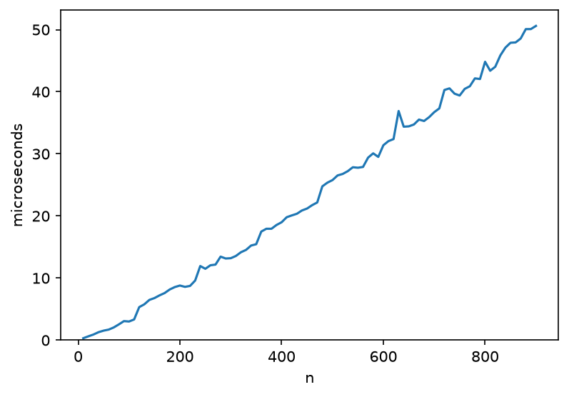

This shape is no surprise. Computing exp(b, n) calls exp a total of n+1 times, and each call performs a roughly fixed amount of work: a comparison, a subtraction, and a multiplication. (Multiplying very large integers does take more work than small ones, but we’ll ignore this difference for now.) The numbers on the vertical axis would differ on another computer, but the shape of the graph would be the same.

The same linear shape emerges if we measure call counts rather than time. Applying the count function from earlier in this section to exp makes every call to exp, including each recursive call, increase exp.call_count. Resetting call_count to 0 before each computation gives the number of calls made to compute exp(2, n) alone.

exp = count(exp)

def calls(n):
    """The number of calls to exp made in computing exp(2, n)."""
    exp.call_count = 0
    exp(2, n)
    return exp.call_count

ns = range(10, 451, 10)
plt.figure(figsize=(6, 4))
plt.plot(ns, [calls(n) for n in ns])
plt.xlabel('n')
plt.ylabel('calls to exp')
plt.ylim(bottom=0)
plt.show()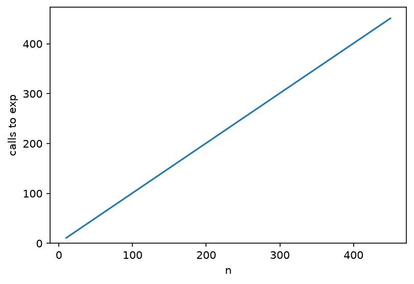

Unlike the timing graph, this graph is a perfectly straight line, and it would be exactly the same on any computer.

Fast Exponentiation. We can compute exponentials in fewer steps by using successive squaring. For instance, rather than computing $b^8$ as

we can compute it using three multiplications:

This method works fine for exponents that are powers of 2. We can also take advantage of successive squaring in computing exponentials in general if we use this recursive rule:

We can express this method as a recursive function as well:

def square(x):
    return x * x

def exp_fast(b, n):
    if n == 0:
        return 1
    elif n % 2 == 0:
        return square(exp_fast(b, n//2))
    else:
        return b * exp_fast(b, n-1)

exp_fast(2, 100)

The graph of the time to compute exp_fast(2, n) has a very different shape. It rises quickly for small values of n and then flattens out. The scale of the vertical axis is different as well: for n of 900, exp_fast is many times faster than exp.

plot_times(lambda n: exp_fast(2, n), range(10, 901, 10))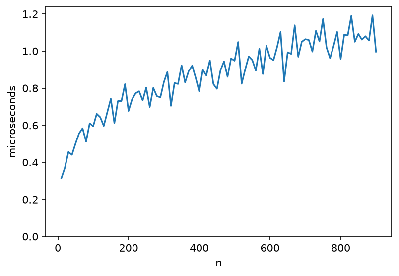

The process evolved by exp_fast grows much more slowly than n because the recursive call often reduces the problem size by half, rather than by 1. The graph is jagged because the number of multiplications depends on more than just the size of n. Each odd exponent along the way involves an extra multiplication, so computing exp_fast(b, 512) requires 10 multiplications, while exp_fast(b, 511) requires 17. But the jaggedness isn’t the important feature. The general shape is important: it shows that very large inputs require only a modest amount of time. This implementation is much more efficient than the previous one.

Measuring call counts rather than time shows a similar shape.

exp_fast = count(exp_fast)

def fast_calls(n):
    """The number of calls to exp_fast made in computing exp_fast(2, n)."""
    exp_fast.call_count = 0
    exp_fast(2, n)
    return exp_fast.call_count

ns = range(10, 901, 10)
plt.figure(figsize=(6, 4))
plt.plot(ns, [fast_calls(n) for n in ns])
plt.xlabel('n')
plt.ylabel('calls to exp_fast')
plt.ylim(bottom=0)
plt.show()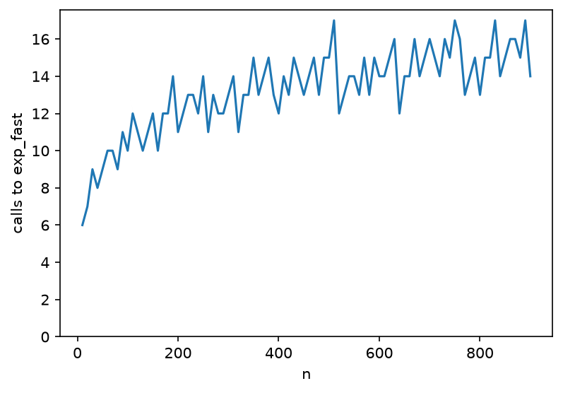

Each call to exp_fast performs at most one multiplication, so this graph also counts multiplications (plus one for the final call with n of 0). It is jagged for the same reason as the timing graph and would be exactly the same on any computer.

Nested processes. When an inner computational process is repeated for each step of an outer process, the time required by the entire process is proportional to the product of the number of steps in the outer and inner processes. For example, the function overlap below counts the pairs of an item in list a and an item in list b that are equal.

def overlap(a, b):
    count = 0
    for item in a:
        for other in b:
            if item == other:
                count += 1
    return count

overlap([3, 5, 7, 6], [4, 5, 6, 5])

If a and b both have length n, then the inner for statement is executed n times, once for each item in a, and each time it compares n pairs of items. So, the expression item == other is evaluated $n \cdot n = n^2$ times. Graphing the time to call overlap on two lists of length n shows that the time grows faster than n: the curve bends upward.

plot_times(lambda n: overlap(list(range(n)), list(range(n))), range(10, 201, 10))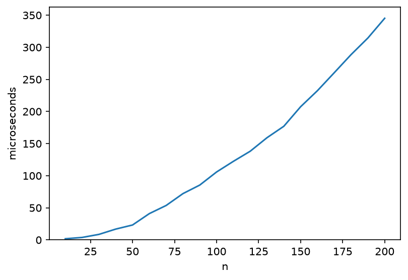

The shape of the curve drawn by graphing a function of the input size for some measurement, such as the running time or number of recursive calls, is the most common way that computer scientists describe the efficiency of a function’s implementation. Specific terminology involving upper and lower bounds is described in Appendix: Orders of Growth for readers who are interested.